Convolutional neural networks (or convnets or CNNs) are a staple of “deep learning”. There are many tutorials available that describe what they do, either mathematically or via quasi-mystical appeals to intuition, and introduce how to train and use them, often with image classification examples.
This post has a narrower focus. As a programmer, I am happy processing floating-point data in languages like C++, but I’m more likely to be building applications with pre-trained models than training new ones. Say I have a pre-trained convnet image classifier, and I use it to carry out a single classification of one image (“tell me whether this shows a pig, cow, or sheep”) — what does that actually mean, in terms of code?
I’ll go through an example in the form of a small hand-written C++ convolutional net that contains only the “execution” code, no training logic. It will be very much an illustrative implementation, not production code. It will use pre-trained data adapted from a similar model in Keras, on which more later.
The specific example I am using is a typical image classification one: identifying which of five types of flower is visible in a small colour image (inspired by this tutorial). All the code I’m describing can be found in this Github repository.
Networks, layers, weights, training
A network in this context is a pipeline of functions through which data is passed, with the output of each function going directly to the input of the next one. Each of these functions is known as a layer.
Our example will begin by supplying the image data as input to the first layer, and end with the final layer returning a set of five numbers, one for each kind of flower the network knows about, indicating how likely the network thinks it is that the image shows that kind of flower.
So to run one classification, we just have to get the image data into the right format and pass it through each layer function in turn, and out pops the network’s best guess.
The layers themselves perform some mathematical operation on the data. Some of them do so by making use of a set of other values, provided separately, which they might multiply with the inputs in some way (in which case they are known as weights) or add to the return values (known as biases).
Coming up with suitable weight and bias values for these layers is what training is for. To train a network, the weights and biases for each such layer are randomly initialised, then the network is repeatedly run to provide classifications of known inputs; each of the network’s guesses is compared with the known class of the input, and the weights and biases of the network are updated depending on how accurate the classification was. Eventually, with luck, they will converge on some reliable values. Training is both difficult and tedious, so here we will happily leave it to machine-learning researchers.
These trainable layers are then typically sandwiched by fixed layers that provide non-linearities (also known as activation functions) and various data-manipulation bits and bobs like max-pooling. More on these later.
The layers are pure functions: a layer with a given set of weights and biases will always produce the same output for a given input. This is not always true within recurrent networks, which model time-varying data by maintaining state in the layers, but it is true of classic convolutional nets.
Our example network
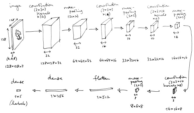
This small network consists of four rounds of convolution + max-pooling layers, then two dense layers.
I constructed and trained this using Keras (in Python) based on a “flower pictures” dataset downloaded from the Tensorflow site, with 5 labelled classes of flowers. My Github repository contains a script obtain-data.sh which downloads and prepares the images, and a Python program with-keras/train.py which trains this network on them and exports the trained weights into a C++ file. The network isn’t a terribly good classifier, but that doesn’t bother me here.
I then re-implemented the model in C++ without using a machine-learning library. Here’s what the pipeline looks like. This can be found in the file flower.cpp in the repository. All of the functions called here are layer functions defined elsewhere in the same file, which I’ll go through in a moment. The variables with names beginning weights_ or biases_ are the trained values exported from Keras. Their definitions can be found in weights.cpp.
vector<float>
classify(const vector<vector<vector<float>>> &image)
{
    vector<vector<vector<float>>> t;

    t = zeroPad(image, 1, 1);
    t = convolve(t, weights_firstConv, biases_firstConv);
    t = activation(t, "relu");
    t = maxPool(t, 2, 2);

    t = zeroPad(t, 1, 1);
    t = convolve(t, weights_secondConv, biases_secondConv);
    t = activation(t, "relu");
    t = maxPool(t, 2, 2);

    t = zeroPad(t, 1, 1);
    t = convolve(t, weights_thirdConv, biases_thirdConv);
    t = activation(t, "relu");
    t = maxPool(t, 2, 2);

    t = zeroPad(t, 1, 1);
    t = convolve(t, weights_fourthConv, biases_fourthConv);
    t = activation(t, "relu");
    t = maxPool(t, 2, 2);

    vector<float> flat = flatten(t);

    flat = dense(flat, weights_firstDense, biases_firstDense);
    flat = activation(flat, "relu");

    flat = dense(flat, weights_labeller, biases_labeller);
    flat = activation(flat, "softmax");

    return flat;
}
Many functions are used for more than one layer — for example we have a single convolve function used for four different layers, with different weights, bias values, and input shapes each time. This reuse is possible because layer functions don’t retain any state from one call to the next.
You can see that we pass the original image as input to the first layer, but subsequently we just take the return value from each function and pass it to the next one. These values have types that we are expressing as nested vectors of floats. They are all varieties of tensor, on which let me digress for a moment:
Tensors
For our purposes a tensor is a multidimensional array of numbers, in our case floats, of which vectors and matrices are special cases. A tensor has a shape, which we can write as a list of sizes, and the length of that list is the rank. (The word dimension can be ambiguous here and I’m going to try to avoid it… apart from that one time I used it a moment ago…)
Examples:
- A matrix is a rank-2 tensor whose shape has two values, height and width. The matrix
has shape
[2, 3], if we are giving the height first. - A C++ vector of floats is a rank-1 tensor, whose shape is a list of one value, the number of elements in the vector. The vector
{ 1.0, 2.0, 3.0 }has the shape[3]. - A single number can also be considered a tensor, of rank 0, with shape
[].
All of the values passed to and returned from our network layer functions are tensors of various shapes. For example, a colour image will be represented as a tensor of rank 3, as it has height, width, and a number of colour channels.
In this code, we are storing tensors using C++ vectors (for rank 1), vectors of vectors (for rank 2), and so on. This is transparent, makes indexing easy, and allows us to see the rank of each tensor directly from its type.
Production C++ frameworks don’t do it this way — they typically store tensors as values interleaved into a single big array, wrapped up in a tensor class that knows how to index into it. With such a design, unlike our code, all tensors will have the same C++ class type regardless of their rank.
There is a practical issue with the ordering of tensor indices. Knowing the shape of a tensor is not enough: we also have to know which index is which. For example, an RGB image that is 128 pixels square has shape [128, 128, 3] if we index the height, width, and colour channels in that order, or [3, 128, 128] if we separate out the individual colour channels and index them first. Unfortunately, both layouts are in common use. Keras exposes the choice through a flag and uses the names channels_last for the former layout, historically the default in Tensorflow as it often runs faster on CPUs, and channels_first for the latter, used by many systems as it parallelises better with GPUs. The code in this example uses channels_last ordering.
This definition of a tensor is good enough for us, but in mathematics a tensor is not just an array of numbers but an object that sits in an algebraic space and can be manipulated in ways intrinsic to that space. Our data structures make no attempt to capture this, just as a C++ vector makes no effort to capture the properties of a mathematical vector space.
Layers used in our model
Each layer function takes a tensor as input, which I refer to within the function as in. Trained layers also take further tensors containing the weights and biases for the layer.
Convolution layer
Here’s the nub of this one, implemented in the convolve function.
for (size_t k = 0; k < nkernels; ++k) {
    for (size_t y = 0; y < out_height; ++y) {
        for (size_t x = 0; x < out_width; ++x) {
            for (size_t c = 0; c < depth; ++c) {
                for (size_t ky = 0; ky < kernel_height; ++ky) {
                    for (size_t kx = 0; kx < kernel_width; ++kx) {
                        out[y][x][k] +=
                            weights[ky][kx][c][k] *
                                in[y + ky][x + kx][c];
                    }
                }
            }
            out[y][x][k] += biases[k];
        }
    }
}
Seven nested for-loops! That’s a lot of brute force.
The weights for this layer, supplied in a rank-4 tensor, define a set of convolution kernels (or filters). Each kernel is a rank-3 tensor, width-height-depth. For each pixel in the input, and for each channel in the colour depth, the kernel values for that channel are multiplied by the surrounding pixel values, depending on the width and height of the kernel, and summed into a single value which appears at the same location in the output. We therefore get an output tensor containing a matrix of (almost) the same size as the input image, for each of the kernels.
(Note for audio programmers: FFT-based fast convolution is not generally used here, as it works out slower for small kernels)
Vaguely speaking, this has the effect of transforming the input into a space determined by how much each pixel’s surroundings have in common with each of the learned kernel patterns, which presumably capture things like whether pixels have a common colour or whether there is common activity between a pixel and neighbouring pixels in a particular direction due to edges or lines in the image.
Usually the early convolution layers in an image classifier will explode the amount of data being passed through the network. In our small model, the first convolution layer takes in a 128×128 image with 3 colour channels, and returns a 128×128 output for each of 32 learned kernels: nearly ten times as much data, which will then be reduced gradually through later layers. But fewer weight values are needed to describe a convolution layer compared with the dense layers we’ll see later in our network, so the size of the trained layer (what you might call the “code size”) is relatively smaller.
I said above that the output matrices were “almost” the same size as the input. They have to be a bit smaller, as otherwise the kernel would overrun the edges. To allow for this, we precede the convolution layer with a…
Zero-padding layer
This can be found in the zeroPad function. It creates a new tensor filled with zeros and copies the input into it:
for (size_t y = 0; y < in_height; ++y) {
    for (size_t x = 0; x < in_width; ++x) {
        for (size_t c = 0; c < depth; ++c) {
            out[y + pad_y][x + pad_x][c] = in[y][x][c];
        }
    }
}
All this does is add a zero-valued border around all four edges of the image, in each channel, in order to make the image sufficiently bigger to allow for the extent of the convolution kernel.
Most real-world implementations of convolution layers have an option to pad the input when they do the convolution, avoiding the need for an explicit zero-padding step. In Keras for example the convolution layers have a padding parameter that can be either valid (no extra padding) or same (provide padding so the output and input sizes match). But I’m trying to keep the individual layer functions minimal, so I’m happy to separate this out.
Activation layer
Again, this is something often carried out in the trained layers themselves, but I’ve kept it separate to simplify those.
This introduces a non-linearity by applying some simple mathematical function to each value (independently) in the tensor passed to it.
Historically, for networks without convolution layers, the activation function has usually been some kind of sigmoid function mapping a linear input onto an S-shaped curve, retaining small differences in a critical area of the input range and flattening them out elsewhere.
The activation function following a convolution layer is more likely to be a simple rectifier. This gives us the most disappointing acronym in all of machine learning: ReLU, which stands for “rectified linear unit” and means nothing more exciting than
if (x < 0.0) {
    x = 0.0;
}
applied to each value in the tensor.
We have a different activation function right at the end of the network: softmax. This is a normalising function used to produce final classification estimates that resemble probabilities summing to 1:
float sum = 0.f;
for (size_t i = 0; i < sz; ++i) {
    out[i] = exp(out[i]);
    sum += out[i];
}
if (sum != 0.f) {
    for (size_t i = 0; i < sz; ++i) {
        out[i] /= sum;
    }
}
Max pooling layer
The initial convolution layer increases the amount of data in the network, and subsequent layers then reduce this into a smaller number of hopefully more meaningful higher-level values. Max pooling is one way this reduction happens. It reduces the resolution of its input in the height and width axes, by taking only the maximum of each NxM block of pixels, for some N and M which in our network are both always 2.
From the function maxPool:
for (size_t y = 0; y < out_height; ++y) {
    for (size_t x = 0; x < out_width; ++x) {
        for (size_t i = 0; i < pool_y; ++i) {
            for (size_t j = 0; j < pool_x; ++j) {
                for (size_t c = 0; c < depth; ++c) {
                    float value = in[y * pool_y + i][x * pool_x + j][c];
                    out[y][x][c] = max(out[y][x][c], value);
                }
            }
        }
    }
}
Flatten layer
Interleaves a rank-3 tensor into a rank-1 tensor, otherwise known as a single vector.
for (size_t y = 0; y < height; ++y) {
    for (size_t x = 0; x < width; ++x) {
        for (size_t c = 0; c < depth; ++c) {
            out[i++] = in[y][x][c];
        }
    }
}
Why? Because that’s what the following dense layer expects as its input. By this point we are saying that we have used as much of the structure in the input as we’re going to use, to produce a set of values that we now treat as individual features rather than as a structure.
With a library that represents tensors using an interleaved array, this will be a no-op, apart from changing the nominal rank of the tensor.
Dense layer
A dense or fully-connected layer is an old-school neural network layer. It consists of a single matrix multiplication, multiplying the input vector by the matrix of learned weights, then a vector addition of bias values. From our dense function:
vector<float> out(out_size, 0.f);

for (size_t i = 0; i < in_size; ++i) {
    for (size_t j = 0; j < out_size; ++j) {
        out[j] += weights[i][j] * in[i];
    }
}

for (size_t j = 0; j < out_size; ++j) {
    out[j] += biases[j];
}
Our network has two of these layers, the second of which produces the final prediction values.
That’s pretty much it for the code. There is a bit of boilerplate around each function, and some extra code to load in an image file using libpng, but that’s about all.
There is one other kind of layer that appears in the original Keras model: a dropout layer. This doesn’t appear in our code because it is only used while training. It discards a certain proportion of the values passed to it as input, something that can help to make the following layer more robust to error when trained.
Further notes
Precision and repeatability
Training a network is a process that involves randomness. A given model architecture can produce quite different results on separate training runs.
This is not the case when running a trained network to make a classification or prediction. Two implementations of a network that both use the same basic arithmetic datatypes (e.g. 32-bit floats) should produce the same results when given the same set of trained weights and biases. If you are trying to reproduce a network’s behaviour using a different library or framework, and you have the same trained weights to use with both implementations, and your results look only “sort of” similar, then they’re probably wrong.
The differences between implementations in terms of channel ordering and indexing can be problematic in this respect. Consider the convolution function with its seven nested for-loops. Load any of those weights with the wrong index or in the wrong order and of course it won’t work, and there are a lot of possible permutations there. There seems to be more than one opinion about how kernel weights should be indexed, for example, and it’s easy to get them upside-down if you’re converting from one framework to another.
Should I use code like this in production?
Probably not!
First and most trivially, this isn’t a very efficient arrangement of layers. Separating out the zero-padding and activation functions means more memory allocation and copying.
Second, there are many ways to speed up the expensive brute-force layers (that is, the convolution and dense layers) dramatically even on the CPU, using vectorisation, careful cache and memory management, and faster matrix and convolution algorithms. If you don’t take advantage of these, you’re wasting time for no purpose; if you do, you’re repeating work other people are doing in libraries already.
I adapted the example network to use the tiny-dnn header-only C++ library, and it ran roughly twice as fast as the code above. (I’m a sucker for libraries named tiny-something, even if, as in this case, they are no longer all that tiny.) That version of the example code can be found in the with-tiny-dnn directory in the repo. It’s ugly, because I had to load and convert the weights from a system that uses channels-last format into one that expects channels-first. But I only had to write that code once, and it wouldn’t have been necessary if I’d trained the model in a channels-first layout. I might also have overlooked some simpler way to do it.
Third, this approach is fragile in the face of changes to the model architecture, which have to be duplicated exactly across the model implementation and the separately-loaded weights. It would be preferable to load the model architecture into your program, rather than load the weights into a hand-written architecture. To this end it seems to make sense to use a library that supports importing and exporting models automatically.
All this said, I find it highly liberating to realise that one could just sketch out these few lines of code and have a working result.
